識別可能性

統計学において、識別可能性とは、正確な推論を可能にするためにモデルが満たさなければならない特性です。モデルは、無限回の観測値を得た後に、そのモデルの基礎となるパラメータの真の値を理論的に学習できる場合、識別可能となります。数学的には、これはパラメータの値が異なると、観測変数の確率分布も異なるものになる、ということと同義です。通常、モデルは特定の技術的制約の下でのみ識別可能であり、その場合、これらの要件の集合は識別条件と呼ばれます。

識別できないモデルは、非識別可能または識別不能であると言われます。つまり、2つ以上のパラメータ化が観測的に同等であるということです。場合によっては、モデルが非識別可能であっても、モデルパラメータの特定のサブセットの真の値を学習することが可能です。この場合、モデルは部分的に識別可能であると言います。また、パラメータ空間の特定の有限領域まで真のパラメータの位置を学習できる場合もあり、その場合、モデルは識別可能とされます。

モデル特性の厳密な理論的な探求とは別に、識別可能性分析を用いてモデルを実験データセットでテストする場合、識別可能性はより広い範囲で参照されることがあります。^[1]

意味

Let ${\displaystyle {\mathcal {P}}=\{P_{\theta }:\theta \in \Theta \}}$ be a statistical model with parameter space ${\displaystyle \Theta }$ . We say that ${\displaystyle {\mathcal {P}}}$ is identifiable if the mapping ${\displaystyle \theta \mapsto P_{\theta }}$ is one-to-one:^[2]

${\displaystyle P_{\theta _{1}}=P_{\theta _{2}}\quad \Rightarrow \quad \theta _{1}=\theta _{2}\quad \ {\text{for all }}\theta _{1},\theta _{2}\in \Theta .}$

This definition means that distinct values of θ should correspond to distinct probability distributions: if θ₁≠θ₂, then also P_θ1≠P_θ2.^[3] If the distributions are defined in terms of the probability density functions (pdfs), then two pdfs should be considered distinct only if they differ on a set of non-zero measure (for example two functions ƒ₁(x) = 1_{0 ≤ x < 1} and ƒ₂(x) = 1_{0 ≤ x ≤ 1} differ only at a single point x = 1 — a set of measure zero — and thus cannot be considered as distinct pdfs).

Identifiability of the model in the sense of invertibility of the map ${\displaystyle \theta \mapsto P_{\theta }}$ is equivalent to being able to learn the model's true parameter if the model can be observed indefinitely long. Indeed, if {X_t} ⊆ S is the sequence of observations from the model, then by the strong law of large numbers,

${\displaystyle {\frac {1}{T}}\sum _{t=1}^{T}\mathbf {1} _{\{X_{t}\in A\}}\ {\xrightarrow {\text{a.s.}}}\ \Pr[X_{t}\in A],}$

for every measurable set A ⊆ S (here 1_{...} is the indicator function). Thus, with an infinite number of observations we will be able to find the true probability distribution P₀ in the model, and since the identifiability condition above requires that the map ${\displaystyle \theta \mapsto P_{\theta }}$ be invertible, we will also be able to find the true value of the parameter which generated given distribution P₀.

Examples

Example 1

Let ${\displaystyle {\mathcal {P}}}$ be the normal location-scale family:

${\displaystyle {\mathcal {P}}={\Big \{}\ f_{\theta }(x)={\tfrac {1}{{\sqrt {2\pi }}\sigma }}e^{-{\frac {1}{2\sigma ^{2}}}(x-\mu )^{2}}\ {\Big |}\ \theta =(\mu ,\sigma ):\mu \in \mathbb {R} ,\,\sigma \!>0\ {\Big \}}.}$

Then

${\displaystyle {\begin{aligned}&f_{\theta _{1}}(x)=f_{\theta _{2}}(x)\\[6pt]\Longleftrightarrow {}&{\frac {1}{{\sqrt {2\pi }}\sigma _{1}}}\exp \left(-{\frac {1}{2\sigma _{1}^{2}}}(x-\mu _{1})^{2}\right)={\frac {1}{{\sqrt {2\pi }}\sigma _{2}}}\exp \left(-{\frac {1}{2\sigma _{2}^{2}}}(x-\mu _{2})^{2}\right)\\[6pt]\Longleftrightarrow {}&{\frac {1}{\sigma _{1}^{2}}}(x-\mu _{1})^{2}+\ln \sigma _{1}={\frac {1}{\sigma _{2}^{2}}}(x-\mu _{2})^{2}+\ln \sigma _{2}\\[6pt]\Longleftrightarrow {}&x^{2}\left({\frac {1}{\sigma _{1}^{2}}}-{\frac {1}{\sigma _{2}^{2}}}\right)-2x\left({\frac {\mu _{1}}{\sigma _{1}^{2}}}-{\frac {\mu _{2}}{\sigma _{2}^{2}}}\right)+\left({\frac {\mu _{1}^{2}}{\sigma _{1}^{2}}}-{\frac {\mu _{2}^{2}}{\sigma _{2}^{2}}}+\ln \sigma _{1}-\ln \sigma _{2}\right)=0\end{aligned}}}$

This expression is equal to zero for almost all x only when all its coefficients are equal to zero, which is only possible when |σ₁| = |σ₂| and μ₁ = μ₂. Since in the scale parameter σ is restricted to be greater than zero, we conclude that the model is identifiable: ƒ_θ1 = ƒ_θ2 ⇔ θ₁ = θ₂.

Example 2

を標準線形回帰モデルとします。 ${\displaystyle {\mathcal {P}}}$

${\displaystyle y=\beta 'x+\varepsilon ,\quad \mathrm {E} [\,\varepsilon \mid x\,]=0}$

（ここで ′ は行列の転置を表す）。このとき、パラメータβ が識別可能であるのは、行列が逆行列である場合のみである。したがって、これがモデルにおける 識別条件である。${\displaystyle \mathrm {E} [xx']}$

例3

古典的な変数誤差線形モデルを仮定します。 ${\displaystyle {\mathcal {P}}}$

${\displaystyle {\begin{cases}y=\beta x^{*}+\varepsilon ,\\x=x^{*}+\eta ,\end{cases}}}$

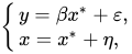
ここで、 ( ε、η、x* ) は期待値がゼロで分散が未知の、互いに正規分布に従う独立なランダム変数であり、変数 ( x、y ) のみが観測される。したがって、このモデルは識別不可能であり、^[4]積 βσ² _∗のみが識別可能である（σ² _∗は潜在回帰変数x*の分散）。これも集合識別可能モデルの一例である。β の正確な値は学習できないが、区間 ( β yx 、 1÷ β xy ) のどこかに収まることは保証できる。_ここで、_β yxはy_のxに対するOLS回帰の係数であり、β _xyはxのyに対するOLS 回帰の係数である。^[5]

正規性仮定を放棄し、x*が 正規 分布しないことを前提とし、独立条件ε⊥η⊥x *のみを保持する と 、モデルは識別可能になる。^[4]

参照

• システム識別
• 構造的識別可能性
• 可観測性
• 同時方程式モデル

参考文献

引用

1. Raue, A.; Kreutz, C.; Maiwald, T.; Bachmann, J.; Schilling, M.; Klingmuller, U.; Timmer, J. (2009-08-01). 「プロファイル尤度を利用した部分観測動的モデルの構造的かつ実用的な識別可能性解析」. Bioinformatics . 25 (15): 1923– 1929. doi : 10.1093/bioinformatics/btp358 . PMID  19505944.
2. Lehmann & Casella 1998, 第1章、定義5.2
3. ファン・デル・ファールト 1998, 62ページ
4. Reiersøl 1950
5. カセラ＆バーガー 2002、583ページ

出典

• Casella, George ; Berger, Roger L. (2002) 『統計的推論』（第2版）、Thomson Learning、ISBN 0-534-24312-6、LCCN  2001025794
• Hsiao, Cheng (1983)、「識別」、計量経済学ハンドブック、第1巻、第4章、North-Holland Publishing Company
• レーマン、EL；カセラ、G.（1998）、点推定理論（第2版）、シュプリンガー、ISBN 0-387-98502-6
• レイエルソル、オラフ（1950）「誤差の影響を受ける変数間の線形関係の識別可能性」、エコノメトリカ、18（4）：375-389、doi：10.2307/1907835、JSTOR  1907835
• van der Vaart、AW (1998)、漸近統計、ケンブリッジ大学出版局、ISBN 978-0-521-49603-2

さらに読む

• Walter, É. ; Pronzato, L. (1997),実験データからのパラメトリックモデルの同定, Springer

計量経済学

• リューベル、アーサー(2019年12月1日). 「識別動物園：計量経済学における識別の意味」 .経済文献ジャーナル. 57 (4). アメリカ経済学会誌: 835–903 . doi :10.1257/jel.20181361. ISSN  0022-0515. S2CID  125792293.
• Matzkin, Rosa L. (2013). 「構造経済モデルにおけるノンパラメトリック同定」. Annual Review of Economics . 5 (1): 457– 486. doi :10.1146/annurev-economics-082912-110231.
• Rothenberg, Thomas J. (1971). 「パラメトリックモデルにおける同定」. Econometrica . 39 (3): 577– 591. doi :10.2307/1913267. ISSN  0012-9682. JSTOR  1913267.