ペアノ核定理

数値解析において、ペアノ核定理は、線形関数を用いて定義される、幅広い数値近似（数値積分法など）の誤差限界に関する一般的な結果である。これはジュゼッペ・ペアノに帰せられる。^[1]

声明

を 上で微分可能で上で有界変分であるすべての関数の空間とし、 を上の線型汎関数とする。が次数の多項式をすべて消滅させると仮定する。すなわち となる。さらに となる任意の2変数関数に対して、次が成り立つとする。のペアノ核をという表記を用いてと定義する。ペアノ核定理^{[1] [2]}によれば、ならばの回連続的に微分可能なすべての関数に対して、次が 成り立つ。${\displaystyle {\mathcal {V}}[a,b]}$ ${\displaystyle f}$ ${\displaystyle (a,b)}$ ${\displaystyle [a,b]}$ ${\displaystyle L}$ ${\displaystyle {\mathcal {V}}[a,b]}$ ${\displaystyle L}$ ${\displaystyle \leq \nu }$ $${\displaystyle Lp=0,\qquad \forall p\in \mathbb {P} _{\nu }[x].}$$ ${\displaystyle g(x,\theta )}$ ${\displaystyle g(x,\cdot ),\,g(\cdot ,\theta )\in C^{\nu +1}[a,b]}$ $${\displaystyle L\int _{a}^{b}g(x,\theta )\,d\theta =\int _{a}^{b}Lg(x,\theta )\,d\theta ,}$$ ${\displaystyle L}$ $${\displaystyle k(\theta )=L[(x-\theta )_{+}^{\nu }],\qquad \theta \in [a,b],}$$ $${\displaystyle (x-\theta )_{+}^{\nu }={\begin{cases}(x-\theta )^{\nu },&x\geq \theta ,\\0,&x\leq \theta .\end{cases}}}$$ ${\displaystyle k\in {\mathcal {V}}[a,b]}$ ${\displaystyle f}$ ${\textstyle \nu +1}$ $${\displaystyle Lf={\frac {1}{\nu !}}\int _{a}^{b}k(\theta )f^{(\nu +1)}(\theta )\,d\theta .}$$

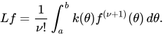
境界

この結果から、の値に関するいくつかの境界が導かれます。${\displaystyle Lf}$ $${\displaystyle {\begin{aligned}|Lf|&\leq {\frac {1}{\nu !}}\|k\|_{1}\|f^{(\nu +1)}\|_{\infty }\\[5pt]|Lf|&\leq {\frac {1}{\nu !}}\|k\|_{\infty }\|f^{(\nu +1)}\|_{1}\\[5pt]|Lf|&\leq {\frac {1}{\nu !}}\|k\|_{2}\|f^{(\nu +1)}\|_{2}\end{aligned}}}$$

ここで、、はそれぞれタクシー、ユークリッドノルム、最大ノルムである。^[2]${\displaystyle \|\cdot \|_{1}}$ ${\displaystyle \|\cdot \|_{2}}$ ${\displaystyle \|\cdot \|_{\infty }}$

応用

実際には、ペアノ核定理の主な応用は、すべての に対して正確な近似値の誤差を制限することです。上記の定理は、整数剰余を持つ に対するテイラー多項式から導かれます。${\displaystyle f\in \mathbb {P} _{\nu }}$ ${\displaystyle f}$

${\displaystyle {\begin{aligned}f(x)=f(a)+{}&(x-a)f'(a)+{\frac {(x-a)^{2}}{2}}f''(a)+\cdots \\[6pt]&\cdots +{\frac {(x-a)^{\nu }}{\nu !}}f^{(\nu )}(a)+{\frac {1}{\nu !}}\int _{a}^{x}(x-\theta )^{\nu }f^{(\nu +1)}(\theta )\,d\theta ,\end{aligned}}}$

を近似値の誤差として定義し、の線形性との正確さを合わせて右辺の最後の項以外を消去し、表記法を使用して積分極限から-依存性を除去します。 ^[3]${\displaystyle L(f)}$ ${\displaystyle L}$ ${\displaystyle f\in \mathbb {P} _{\nu }}$ ${\displaystyle (\cdot )_{+}}$ ${\displaystyle x}$

参照

• 相違点の分割

参考文献

1. Ridgway Scott, L. (2011).数値解析. プリンストン大学出版局, ニュージャージー州, 209頁. ISBN 9780691146867. OCLC  679940621。
2. Iserles, Arieh (2009). 『微分方程式の数値解析入門』（第2版）. ケンブリッジ: ケンブリッジ大学出版局. pp. 443–444. ISBN 9780521734905. OCLC  277275036。
3. Iserles, Arieh (1997). 「数値解析」(PDF) . 2018年8月9日閲覧。